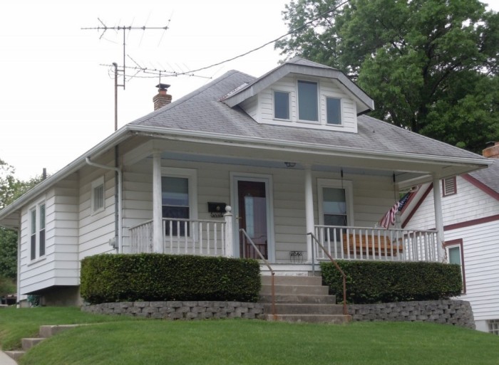
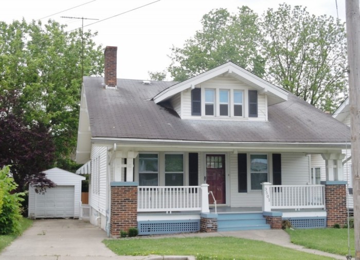
In [1]:
from IPython.display import HTML  # for hiding code cells
In [2]:
HTML('''<script>
code_show=true; 
function code_toggle() {
 if (code_show){
 $('div.input').hide();
 } else {
 $('div.input').show();
 }
 code_show = !code_show
} 
$( document ).ready(code_toggle);
</script>
The computer code for this report is by default hidden for easier reading.
To toggle the code on and off, click <a href="javascript:code_toggle()">here</a>.''')
Out[2]:
The computer code for this report is by default hidden for easier reading. To toggle the code on and off, click here.

Sears Roebuck Kit Home Report

M. Fawcett - December 23, 2021
rev. 01/21/2022

A Short History of Sears Kit Homes

Between 1908 and 1942, the Sears Roebuck company sold houses in the form of build-it-yourself kits. Huge kits were prepared at factories, mostly in Illinois, and shipped in railroad freight cars to customers all over the country. Each kit contained all the materials needed to build a house. Customers lugged their 25 tons of numbered precut lumber, shingles, wall board, flooring and so on, from the freight car to their building site, and got to work following the instructions in the 75 page construction guide. Happy buyers considered the homes attractive, well designed and economical, about 30 percent less costly than a similar, existing home.

For me personally, this business model seems crazy and impractical, but Sears wasn't the only one selling kit homes. They were the most successful however, selling between 75,000 and 100,000 of them. Because Sears was a mail-order marketer of all manner of merchandise, they also sold the tools used to build the houses, and then the appliances, furniture and fixtures that filled them when they were completed. More than one observer has called Sears the Amazon of its time.

But success got cut short when the Great Depression and World War II took away much of the demand for new housing. After World War II a new trend in housing, tract housing, took over and the Sears kit home business faded into oblivion. The Sears company itself has lately been fading into oblivion. Having declared bankruptcy in 2018, Sears barely exists at all now except in legal proceedings while its few remaining stores are gradually liquidated.

With no official list of where the kit homes were built, a few fascinated enthusiasts now hunt for them and share their discoveries through social media and Websites. They find the story of these homes so appealing that they don't want to see them lost to history.

This report describes where kit homes have been found and offers clues as to where others are likely to be be found. It will look at things like street name, distance from railroads, local economic factors and population characteristics.

This report was written in the Python computer language. (There is a link at the top of the report for hiding or showing the computer code.) Another software program called QGIS was used to prepare some of the data displayed in the maps. The US Census Bureau provided neighborhood social and economic data.

Summary

This report confirms some fan beliefs about where to find Sears kit homes. Based on the analysis of kit homes in Ohio, I found,

  1. Certain street names, such as early presidents and trees, tend to have more kit homes.
  2. Kit homes tend to be within 1 or 2 miles of a railroad track.
  3. Ohio has the most known kit homes, followed by Illinois, Pennsylvania and New York.
  4. Kit homes are more likely to be in areas where the US Census Bureau reports a higher percentage of dwellings built prior to 1940.
  5. Kit homes tend to be found in areas where household income is lower than the state overall.
  6. Kit homes tend to be in areas with a higher proportion of rental properties than the state overall.

Education level and population age do not seem to be associated with areas havong greater numbers of kit homes.

Below there are a couple of interactive maps that let you zoom into a view of the US to see where kit homes are located. With a few extra mouse clicks you can see a picture of the home in Google Street View.

My original goal when starting this project was to create a computer program that could analyze a picture of a house and determine if it was a Sears kit home. This turned out to be too hard a problem due to the large number of different looking models (over 350) produced over the years. Another goal was to have the computer program methodically "crawl" through Google Street View images and pick out houses that had a high probability of being a Sears kit home. This turned out to be impractical because Google charges 7/10ths of a cent every time a computer program uses Street View to capture an image. The bill for scanning 10,000 images was \$70.00. Scanning 1 million images would have cost \\$7,000.00.

In [3]:
%%capture --no-display  
# Previous line supresses a warning about package versioning
# Load Python modules needed for the analysis
import pandas as pd   # for dataframe manipulation
import numpy as np  # for numerical analysis
import matplotlib.pyplot as plt   # for generating plots and graphs
from matplotlib.pyplot import figure  # for modifying appearance of plots & graphs
import requests   # to make http post requests to the US Census geocoder
import io  # for working with I/O streams and allow conversion of geocode response to dataframe 
import csv  # reading/writing csv files
import pickle as pk # to store and retrieve dataframes on disk
import csv  # to read text files
import requests # to make http requests for data using census web API
import os   # to list contents of disk drive folders
import sys  # for managing system options
import folium  # the mapping package
from folium import plugins  # to allow cluster markers on maps
import seaborn as sns   # for fancy plotting
from IPython.display import Markdown as md  # for embedding variables in markdown cells
from IPython.display import Image   # to embeg jpg images in notebook
In [4]:
# See http://blog.nextgenetics.net/?e=102 for hiding computer code in this report.
# For internal links table of contents see...
# https://nbviewer.org/github/rasbt/python_reference/blob/master/tutorials/table_of_contents_ipython.ipynb#top
In [5]:
# Settings to improve the display of tabular results
pd.set_option('display.max_columns', None)
pd.set_option('display.max_rows', None)
np.set_printoptions(threshold = sys.maxsize)

In [62]:
HTML('''<script>
code_show=true; 
function code_toggle() {
 if (code_show){
 $('div.input').hide();
 } else {
 $('div.input').show();
 }
 code_show = !code_show
} 
$( document ).ready(code_toggle);
</script>
The computer code for this report is by default hidden for easier reading.
To toggle the code on and off, click <a href="javascript:code_toggle()">here</a>.''')
Out[62]:
The computer code for this report is by default hidden for easier reading. To toggle the code on and off, click here.

Preparing the Data [Contents]

A spreadsheet (maintained by LS) of around 13,000 kit home locations is the basis of this analysis. The list of locations is as of October 27,2021.

The first step was to load the list of kit home addresses from the spreadsheet into computer memory and do some minor tidying of the data. Overall the spreadsheet data is pretty clean. The values in each column were entered in a consistent way so there was not a need to do much cleanup to make good use of the data.

The main cleanup was in a column called "Auth?". I changed the name to "Auth" and all the values in the column were converted to uppercase so they are either "YES" or "NO". The Auth column indicates whether a location has gone through a confirmation step showing there is evidence that it is truly a Sears kit home.

Below is a sample of the data from the spreadsheet after the cleanup.

None of the cleanup effected the original spreadsheet. All of this work is done on an in-memory copy of the spreadsheet data.

In [6]:
# Read the Excel file of kit home locations into a Pandas dataframe.
address_df = pd.read_excel(r"Sears Roebuck Houses.xlsx", sheet_name = "Locations")

# Add a row number to each address.  A unique number for each row will be needed by the 
# US Census Bureau geocoder
address_df.insert(loc=0, column='row_num', value=np.arange(len(address_df)) + 2) 
# the +2 is to add 2 to each row number to account for the header row and row "0".
# I want the row_num value to be aligned wth the row number in the original Excel file.

# Remove the "?" from the Auth? column name.
address_df.rename(columns={"Auth?": "Auth"}, inplace = True)

# Tidy up the values in the "Auth" column
# Change the "nan" to "N/A".
address_df["Auth"] = address_df["Auth"].replace(np.nan, 'N/A', regex=True)
# Make all the values in the Auth? column uppercase
address_df["Auth"] = address_df["Auth"].apply(lambda x: x.upper())

# Examine some of the cleaned up data
address_df.head()
Out[6]:
row_num Model Address City State Year Auth Added Notes Link #1 Link #2 Twp/Borough/Neighborhood County and State
0 2 Windsor 105 Meadow Brook Dr Clarks Summit PA NaN NO AIM NaN NaN NaN NaN NaN
1 3 Columbine 11146 66 St NW Edmonton AB 1928.0 YES LS Building permit. Canada NaN NaN NaN NaN
2 4 Belmont (old one) 541 Pine St Ketchikan AK NaN NO LS NaN NaN NaN NaN NaN
3 5 Americus 303 E Samford Ave Auburn AL NaN NO NaN NaN http://photos.al.com/alphotos/2014/09/alabamas... NaN NaN NaN
4 6 Elsmore 608 Brummel Ave Bridgeport AL NaN NO NaN NaN NaN NaN NaN NaN
In [7]:
# Total number of locations
tot = len(pd.unique(address_df["Address"]))
# Number authenticated
yes_n = len(address_df[address_df["Auth"] == 'YES'])
md("The total number of locations contained in the spreadsheet is {:,}. The number that have been authenticated is {:,}.".format(tot, yes_n))
Out[7]:

The total number of locations contained in the spreadsheet is 13,832. The number that have been authenticated is 5,688.

Count of Kit Homes by State [Contents]

As the chart below shows, Ohio has the most kit homes followed by Illinois, Pennsylvania and New York. Every state appears to have at least one kit home.

These counts include authenticated plus unauthenticated locations.

In [8]:
state_count = address_df['State'].value_counts() 

# Plot a barchart 
figure(figsize=(16, 6))
state_count.plot.bar()
plt.title("Number of Locations by State")
plt.show()

Count of Kit Homes by Model Name [Contents]

In [9]:
num_models = len(address_df['Model'].value_counts())

md("There are {} models mentioned in the spreadsheet. Some of these are variations "  \
      "of the same model name, for example Concord, Concord/No. 114, Concord/No. 3379.".format(num_models))
Out[9]:

There are 432 models mentioned in the spreadsheet. Some of these are variations of the same model name, for example Concord, Concord/No. 114, Concord/No. 3379.

In [10]:
# List all the model names in alphabetical order.
models_df = pd.DataFrame(pd.unique(address_df["Model"])) # .astype(str).sort())
# models_df[0].sort_values()

Below is a list of the 50 most frequently mentioned model names in the spreadsheet and how many times each was mentioned.

In [11]:
model_count = address_df['Model'].value_counts().nlargest(50) 

# Plot a barchart 
figure(figsize=(10, 16))
model_count.plot.barh()
plt.title("Number of Kit Homes by Model Name (Top 50)")
plt.show()

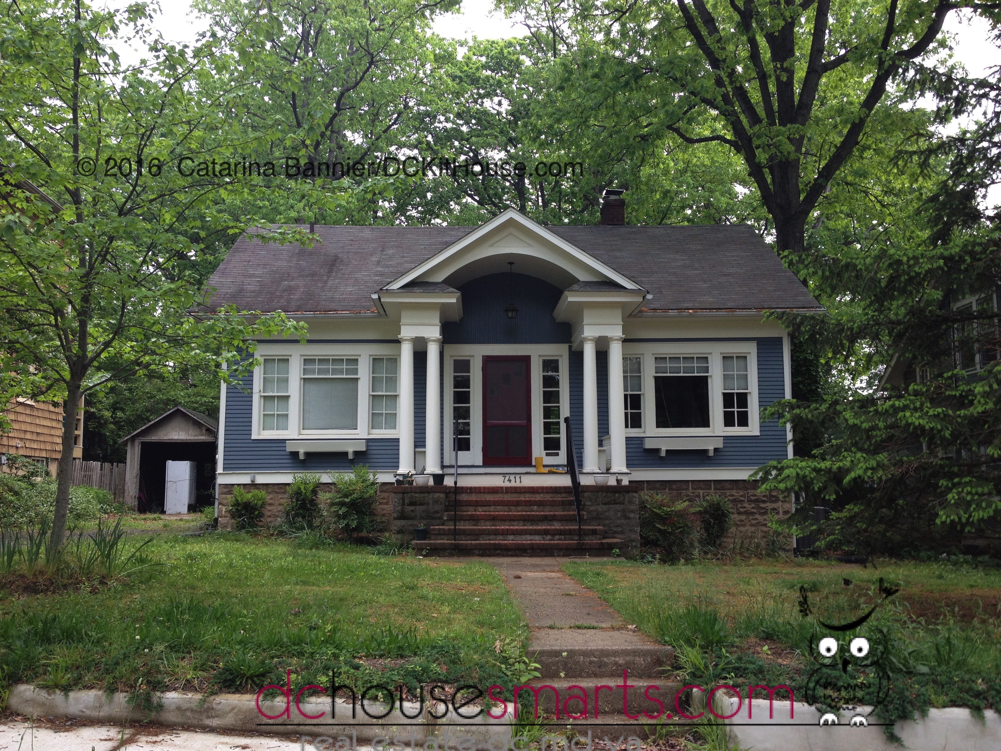
Pictures of Crescent, Startlight and Vallonia Models.

Below are pictures of the three models that appear most frequently in the spreadsheet data.
Drawing
Crescent
Drawing
Startlight
Drawing
Vallonia

Geocoding addresses [Contents]

Mapping the kit home locations requires having their longitude and latitude. The US Census Bureau provides a service called "Geocoding" for translating a mailing address into a pair of long/lat coordinates. It took around 20 minutes to process the list of 13,000 addresses using the Census Bureau service. There was no charge for this. Not every attempt at geocoding will result in an exact match, but in most cases here, it did.

Below is a sample of the spreadsheet data enhanced with the additional information provided by the geocoding. Scrolling the sample horizontally reveals the additional columns for longitude, latitude, state code, county code and census tract number and Zip Code. More about "census tracts" and "GEOIDs" later.

In [12]:
# Retrieve the coordinates and other results of the geocoding that were previously stored in a computer file.
geocoded_results_df = pd.read_pickle('geocoded_results.pkl')

# Only keep rows that were successfully geocoded
geocoded_results_df = geocoded_results_df[geocoded_results_df["MATCH_INDICATOR"] == "Match"]

# Convert geography code values from numeric to string
geocoded_results_df['FIPS_STATE'] = geocoded_results_df['FIPS_STATE'].astype(int).astype(str)
geocoded_results_df['FIPS_COUNTY'] = geocoded_results_df['FIPS_COUNTY'].astype(int).astype(str)
geocoded_results_df['CENSUS_TRACT'] = geocoded_results_df['CENSUS_TRACT'].astype(int).astype(str)

# Left pad geograpgy values wit zeros
geocoded_results_df['FIPS_STATE'] = geocoded_results_df['FIPS_STATE'].apply('{:0>2}'.format)
geocoded_results_df['FIPS_COUNTY'] = geocoded_results_df['FIPS_COUNTY'].apply('{:0>3}'.format)
geocoded_results_df['CENSUS_TRACT'] = geocoded_results_df['CENSUS_TRACT'].apply('{:0>6}'.format)


# Create a unique geographic identifier by combining state, county and cenus tract code for each row.
geocoded_results_df["GeoID"] = geocoded_results_df["FIPS_STATE"] \
                                + geocoded_results_df["FIPS_COUNTY"] \
                                + geocoded_results_df["CENSUS_TRACT"]

# Split the LONG_LAT column into separate Longitude and Latitude columns
geocoded_results_df[['Longitude', 'Latitude']] = geocoded_results_df['LONG_LAT'].str.rsplit(',', 1, expand=True)

# Merge the Sears Kit Home style for each location from the original address list with the geocoded results.
mapping_data_df = pd.merge(left = address_df[['row_num','Model','Address','City','State','Auth']], 
                           right = geocoded_results_df, 
                           how = 'right', 
                           left_on = 'row_num',
                           right_on = 'ID')

# Examine some of the results
mapping_data_df.head()
Out[12]:
row_num Model Address City State Auth ID ADDRESS_IN MATCH_INDICATOR MATCH_TYPE ADDRESS_OUT LONG_LAT TIGER_EDGE STREET_SIDE FIPS_STATE FIPS_COUNTY CENSUS_TRACT CENSUS_BLOCK Zipcode GeoID Longitude Latitude
0 2 Windsor 105 Meadow Brook Dr Clarks Summit PA NO 2 105 Meadow Brook Dr, Clarks Summit, PA, Match Exact 105 MEADOW BROOK DR, CLARKS SUMMIT, PA, 18411 -75.71287,41.500095 139319156.0 R 42 069 110402 2006.0 18411 42069110402 -75.71287 41.500095
1 4 Belmont (old one) 541 Pine St Ketchikan AK NO 4 541 Pine St, Ketchikan, AK, Match Exact 541 PINE ST, KETCHIKAN, AK, 99901 -131.64699,55.344284 207096132.0 L 02 130 000300 2000.0 99901 02130000300 -131.64699 55.344284
2 5 Americus 303 E Samford Ave Auburn AL NO 5 303 E Samford Ave, Auburn, AL, Match Exact 303 E SAMFORD AVE, AUBURN, AL, 36830 -85.47823,32.59884 1569988.0 L 01 081 040300 2008.0 36830 01081040300 -85.47823 32.59884
3 6 Elsmore 608 Brummel Ave Bridgeport AL NO 6 608 Brummel Ave, Bridgeport, AL, Match Exact 608 BRUMMEL AVE, BRIDGEPORT, AL, 35740 -85.7156,34.947346 58044064.0 R 01 071 950200 1062.0 35740 01071950200 -85.7156 34.947346
4 7 Osborn 708 2nd St SE Cullman AL NO 7 708 2nd St SE, Cullman, AL, Match Exact 708 2ND ST SE, CULLMAN, AL, 35055 -86.83624,34.17931 130220321.0 R 01 043 964901 4032.0 35055 01043964901 -86.83624 34.17931
In [13]:
# Build a list containing all the coordinates so they be plotted on the map
locations = mapping_data_df[['Latitude', 'Longitude']]
locationlist = locations.values.tolist()

How to use the interactive map [Contents]

The map below shows the CONFIRMED (authenticated) kit homes using DARK BLUE markers and the UNCONFIRMED (not authenticated) kit homes using LIGHT BLUE markers.

The icon that looks like a stack of square pancakes in the upper right corner of the map is the "layer control". You can use it to hide or show the confirmed and unconfirmed markers.

The + and - icons in the upper left of the map lets you zoom in and out. If your mouse has a wheel, you can use it to zoom. If you have a track pad you may be able to swipe it to zoom as well.

The numbers in the blue rectangles represent the number of houses in the group it represents. Clicking on a numbered marker zooms in and separates the big group into smaller groups. The groups themselves don't mean anything. They are just there to make the map look less cluttered instead of displaying thousands of markers. There is no way to turn off grouping to see all the individual markers at once.

Once you zoom in far enough you will see individual markers that tag a single location. These are the markers with a little "i" in the center. If you click on one of these you will see the address, the model name and whether it has been confirmed.

Something that is kind of fun to do is to highlight the address (just the address) in the pop-up tag, right-click the highlight, and select "Search with Google" (it might say something different depending on your browser). In most cases it will bring up a Google Street View page for the house. There is no charge for this sort of use of Street View.

Map of Kit Home Locations [Contents]

In [14]:
### Define functions to set the color of cluster markers. Confirmed and unconfirmed locations have 
### different colors. This gets used by all maps.
# This sets the color for CONFIRMED locations clusters.
icon_create_function_confirmed = """
    function(cluster) {
    var childCount = cluster.getChildCount(); 
    /* 
    // comment: can have something like the following to modify the different cluster sizes....
    var c = ' marker-cluster-';

    if (childCount < 50) {
        c += 'large';
    } else if (childCount < 300) {
        c += 'medium';
    } else {
        c += 'small';
    }    
    
    // The marker-cluster-<'size'> gets passed in the "return new L.DivIcon()" function below.
    */
    
    return new L.DivIcon({ html: '<div><span style="background-color:darkblue;color:white;font-size: 20px;">' + childCount + '</span></div>', className: 'marker-cluster', iconSize: new L.Point(40, 30) });    
    }
    """

# This sets the color of UNCONFIRMEDlocation clusters.
icon_create_function_unconfirmed = """
    function(cluster) {
    var childCount = cluster.getChildCount(); 

    return new L.DivIcon({ html: '<div><span style="background-color:lightblue;color:black;font-size: 20px;">' + childCount + '</span></div>', className: 'marker-cluster', iconSize: new L.Point(40, 30) });    
    }
    """
In [15]:
# Create a map using the Map() function and the coordinates of the locations of all the homes.

# Map starts out centered on Ohio.
mp = folium.Map(location=[40.367474, -82.996216], zoom_start=7, width=900, height=550, control_scale=True)
# Ohio_map


# Feature groups allow customization of layer control labels so they don't have to say "macro blah...""
fg_confirmed = folium.FeatureGroup(name = 'Confirmed Locations', show = True)
mp.add_child(fg_confirmed)
fg_unconfirmed = folium.FeatureGroup(name = 'Unconfirmed Locations', show = True)
mp.add_child(fg_unconfirmed)

# Add the Marker clusters for confirmed and unconfirmed locations to feature group
marker_cluster_confirmed = plugins.MarkerCluster(icon_create_function = icon_create_function_confirmed).add_to(fg_confirmed)  
marker_cluster_unconfirmed = plugins.MarkerCluster(icon_create_function=icon_create_function_unconfirmed).add_to(fg_unconfirmed) 

# A function to choose a marker color depending on if the house is a confirmed kit house or not.
# The individual location markers use the same color as their cluster markers.
def getcolor(auth_val):
    if auth_val == 'YES':
        return ("darkblue", "Confirmed")
    return ("lightblue","Unconfirmed")

### Add a layer to the map shpwing Confirmed kit homes
# Loop through all ther location pairs.
for point in range(0, len(locationlist)):
    try:
        clr, status = getcolor(mapping_data_df["Auth"][point])
        if status == "Confirmed":
            folium.Marker(
                location = locationlist[point], 
                popup = status + " " + mapping_data_df['Model'][point] + ": " + mapping_data_df['ADDRESS_OUT'][point],            
                icon = folium.Icon(color = clr)
            ).add_to(marker_cluster_confirmed)

    except Exception:  # not all addresses could be geocoded so skip them if coordinates are missing
        pass
        
### Add a layer to the map showing Unconfirmed kit homes
for point in range(0, len(locationlist)):
    try:
        clr, status = getcolor(mapping_data_df["Auth"][point])
        if status == "Unconfirmed":
            folium.Marker(
                location = locationlist[point], 
                popup = status + " " + mapping_data_df['Model'][point] + ": " + mapping_data_df['ADDRESS_OUT'][point],            
                icon = folium.Icon(color = clr)
            ).add_to(marker_cluster_unconfirmed)

    except Exception:  # not all addresses could be geocoded so skip them if coordinates are missing
        pass
        
# add layer control to map (allows layer to be turned on or off)
folium.LayerControl().add_to(mp)

# Display the map
mp
Out[15]:
Make this Notebook Trusted to load map: File -> Trust Notebook

Most Frequent Street Names [Contents]

There are anectdotal reports that certain street names are more likely to have kit homes. This might be caused if trends in street naming occur over time and certain street names were more popular before 1942, when the last kit home was sold. To see if there is data to support this, I looked at the distribution of kit homes on Ohio street names and it turns out that it seems to be true. One conclusion from this data would be to look for streets named for presidents who came before Franklin Roosevelt. Also look for streets named for aspects of nature, like trees and flowers.

I started by counting the number of residential addresses for each street name in Ohio. Dividing the count for each street name by the total number of residential addresses in Ohio gives a proportion for each street. I did a similar calculation using the number of kit homes on each street name and the total number of kit homes in Ohio. Then I compared the two proportions for each street name. If a street's proportion in the kit home calculation was greater than the proportion for residential addresses overall, it might indicate that a street name is more likely to have a kit home on it.

For the proportion calculations I used both the authenticated and unauthenticated locations. Street names were converted to the base version of the actual street name, without adornments like "DR", "AVE", "N", "S" etc. I did not convert numbered streets like "1st" to "First", which might have improved the results a bit.

To get the number of residential addresses for each street I used a resource called the National Address Database maintained by the US Department of Transportation. See https://www.transportation.gov/gis/national-address-database/national-address-database-0.

In [16]:
# Build an Ohio list of kit house locationss
kitpoints_df = mapping_data_df.loc[(mapping_data_df['MATCH_INDICATOR'] != 'No_Match') & (mapping_data_df['State'] == 'OH'), ['Model', 'Latitude', 'Longitude', 'FIPS_STATE', 'FIPS_COUNTY', 'CENSUS_TRACT', 'GeoID']] # ['Model', 'Latitude', 'Longitude']]
num_kithomes_in_state = len(kitpoints_df)
In [17]:
# Save the Ohio points to a csv file so the data can be used by QGIS software later.
kitpoints_df.to_csv("OhioKitPoints.csv", sep = ",", header = True, index = False)
In [18]:
# The next step assumes that I previously downloaded the street addresses for Ohio from the National Address Database 
# and stored them in a CSV file.
# Extract the street name and address type of each address in the state from the csv file.
column_lst = ["StreetName", "Addr_Type"]
nad_addressTypes_df = pd.read_csv("NAD_r7_Ohio.csv", usecols = column_lst)
# Count the occuraces of each address type
addrtype_df = pd.DataFrame(nad_addressTypes_df.groupby(['Addr_Type']).size())

# Assign name to column containing counts
addrtype_df.rename(columns={0: "Count"}, inplace = True)

These are the counts for the different address types in Ohio according to the NAD.

In [19]:
addrtype_df
Out[19]:
Count
Addr_Type
Commercial 286354
Educational 1898
Government 1413
Industrial 735
Other 22863
Residential 3501707
Unknown 854263
In [20]:
state_address_count = addrtype_df.loc["Residential", "Count"] 

md("There are {:,} addresses that are specifically identified as Residential in Ohio according to the \
NAD. I will use {:,} as the denominator when calculating the proportion of residential addresses on each \
street name.  There are {:,} Ohio kit homes in the spreadsheet.".format(state_address_count,state_address_count, num_kithomes_in_state))
Out[20]:

There are 3,501,707 addresses that are specifically identified as Residential in Ohio according to the NAD. I will use 3,501,707 as the denominator when calculating the proportion of residential addresses on each street name. There are 2,745 Ohio kit homes in the spreadsheet.

In [21]:
# The NAD "StreetName" column provides a basic (without Drive, Street, Avenue, etc) street name for 
# each address, which is what I'll need in my street address frequency analysis.
nad_street_address_count_df = pd.DataFrame(nad_addressTypes_df.loc[nad_addressTypes_df['Addr_Type'] == 'Residential'].groupby(['StreetName']).size().sort_values(ascending=False))
In [22]:
# Getting a similar basic street name for each address in the kit home list is a little more complicated.

# Start with the full addresses
kithome_address_df = mapping_data_df.loc[mapping_data_df['State'] == 'OH', ("State", 'Address')]

# Remove anything that is not a word character or a space
myregex0 = r"[^\w\s]"
kithome_streetnames_ser0 = kithome_address_df["Address"].str.replace(myregex0, '', regex = True, case = False)

# Replace the leading number wih the word ""
myregex1 = r"(^\d+)"
kit_home_streetnames_ser1 = kithome_streetnames_ser0.str.replace(myregex1, '', regex = True, case = False)

# Remove N, E, S, W, St, Ave, Rd, Dr
myregex2 = r"( [nesw]\b)|( dr\b)|( st\b)|( rd\b)|( ave\b)|( pl\b)|( blvd\b)|( se\b)|( ne\b)"
kithome_streetnames_ser2 = kit_home_streetnames_ser1.str.replace(myregex2, '', regex = True, case = False)

num_kithomes_in_state = len(kithome_streetnames_ser2)

To keep things managable I'll focus on 30 street names with the most kit homes.

In [23]:
# Count the kit homes per street and take the top 30 streets.
kithome_top_30_streets_df = pd.DataFrame(kithome_streetnames_ser2.value_counts()).head(30)

# Give the counts column a name
kithome_top_30_streets_df.columns = ["Actual Kit Homes"]

# Give the index a name
kithome_top_30_streets_df.index.name = "StreetName"

# Make index upper case
kithome_top_30_streets_df.index = kithome_top_30_streets_df.index.str.upper()

# Strip whitespace off index values (the street names)
kithome_top_30_streets_df.index = kithome_top_30_streets_df.index.str.strip()
In [24]:
# Get the address count proportions for street names in state overall
ohio_address_count_by_street_df = nad_street_address_count_df

# Add a column heading
ohio_address_count_by_street_df.columns = ["AddressCount"]

# A# Add a column that shows the proportion of addresses for each street in the state 
ohio_address_count_by_street_df['Proportion'] = ohio_address_count_by_street_df['AddressCount'] / state_address_count
In [25]:
md("The table below is a list of street names where the actual number of kit homes exceeded the \
expected number of kit homes. For example, in the first row, for streets named Park there were a total of \
9,700 residential addresses. It represents 0.002770 of all the residential addresses in Ohio {:,}.".format(state_address_count))
Out[25]:

The table below is a list of street names where the actual number of kit homes exceeded the expected number of kit homes. For example, in the first row, for streets named Park there were a total of 9,700 residential addresses. It represents 0.002770 of all the residential addresses in Ohio 3,501,707.

In [26]:
md("You might expect a similar proportion of the {:,} Ohio kit homes to be located on a street named Park. \
That works out to be 7.60. The data shows there are actually 9 homes.  Whether any of these results are \
statistically significant is not something I can say. Also, these results are just for one state but \
it shows it could be worthwhile to expand the street analysis to the rest of the country.".format(num_kithomes_in_state))
Out[26]:

You might expect a similar proportion of the 2,745 Ohio kit homes to be located on a street named Park. That works out to be 7.60. The data shows there are actually 9 homes. Whether any of these results are statistically significant is not something I can say. Also, these results are just for one state but it shows it could be worthwhile to expand the street analysis to the rest of the country.

In [27]:
# Calculate the number of kits homes expected for each Ohio Street
ohio_address_count_by_street_df["Expected Kit Homes"] = round(ohio_address_count_by_street_df["Proportion"] * num_kithomes_in_state, 2)

# Merge the actual counts of kit homes by street name and compare to the expected number.
comparison3_df = ohio_address_count_by_street_df.join(kithome_top_30_streets_df, lsuffix='_State', rsuffix='_Kits')


comparison3_df[comparison3_df["Actual Kit Homes"] - comparison3_df["Expected Kit Homes"] > 0]
Out[27]:
AddressCount Proportion Expected Kit Homes Actual Kit Homes
StreetName
PARK 9700 0.002770 7.60 9.0
MAPLE 9136 0.002609 7.16 15.0
WASHINGTON 9030 0.002579 7.08 9.0
LINCOLN 8373 0.002391 6.56 9.0
CLEVELAND 6511 0.001859 5.10 16.0
BROADWAY 6103 0.001743 4.78 9.0
OAK 5713 0.001631 4.48 10.0
CHURCH 5176 0.001478 4.06 9.0
RIVER 4544 0.001298 3.56 13.0
FOREST 2986 0.000853 2.34 9.0
WARREN 2182 0.000623 1.71 12.0
CAMBRIDGE 1838 0.000525 1.44 17.0
WOOSTER 1721 0.000491 1.35 11.0
HUNTER 1103 0.000315 0.86 10.0
HILLSIDE 885 0.000253 0.69 12.0
WYOMING 855 0.000244 0.67 10.0
SEYMOUR 539 0.000154 0.42 8.0
SUTTON 472 0.000135 0.37 11.0
BEACON 415 0.000119 0.33 13.0
JOSEPH 391 0.000112 0.31 9.0
PONDVIEW 181 0.000052 0.14 9.0
CARTHAGE 145 0.000041 0.11 10.0
FOURTEENTH 137 0.000039 0.11 14.0
ELBERON 86 0.000025 0.07 9.0
KRYDER 49 0.000014 0.04 9.0
HOLLIBAUGH 48 0.000014 0.04 9.0

Distance to railroad [Contents]

Sears kit homes were delivered from the factory by railroad freight car. Areas closer to railroads may be more likely to have kit homes due to the effort and expense involved in moving the materials from the railroad to the building site.

The US Census Bureau provides mapping files for railroad tracks. Using QGIS geospatial software I calculated the shortest distance between every kit home and the nearest railroad track. Then I calculated what percentage of kit homes were found with a mile, two miles etc, of railroad tracks. I used Ohio as the test for this.

In [28]:
# Analyze the distances that were found.  The distances are Euclidean distance, or "as the crow flies" 
# distance between a house and the nearest railroad track.  It ignores whether the nearest RR found is at a 
# spur or yard where unloading could actually take place.

# Load the CSV file contianing the distance measures.
distances_df = pd.read_csv("~/Documents/CensusUS/Hub Distances.csv")

The following chart shows that in Ohio a large majority of the kit homes are within one or two miles of a railroad track. 63 percent are within 1 mile of a railroad. 79 percent are within 2 miles of a railroad.

In [29]:
plt.figure(figsize=(12, 5))
my_bins = [0, 1, 2, 3, 4, 5, 6, 7, 8, 9, 10, 11, 12]
arr = plt.hist(distances_df["HubDist"], bins = my_bins)
plt.xticks([0,1,2,3,4,5,6,7,8,9,10,11,12])

for i in range(len(my_bins) - 1):
    plt.text(x = arr[1][i] + 0.2, y = arr[0][i] + 15, s = str(int(arr[0][i])), fontsize = 12)
    # plt.xlabel('Value')

plt.ylabel('Number of Houses')
plt.xlabel('Range of Distances to Nearest Railroad - Miles')

plt.show()
In [30]:
# Create a dataframe of the cummulative percents for each bin of distance
lst = []  # list object to hold the rows of calculations
cummul = 0
for i in range(len(my_bins) - 1):    
    cummul = cummul + int(arr[0][i])
    # Append the row of calculations to the main ;ist 
    lst.append([str(i) + ' to ' + str(i + 1), int(arr[0][i]), cummul, round(cummul / len(distances_df), 3) * 100])
    
# Create the DataFrame from the list of calculations
distance_df = pd.DataFrame(lst , columns = ['Distance to RR in Miles', 'Count', 'Cummulative Count', 'Cummulative Percent'])

Using Distance to Railroad Track for Prediction

The Census Bureau provides the longitude and latitude of the geocentric center of census tracts. I used those points in a QGIS map layer to find the distance to railroad tracks.

The shaded areas on the map are the census tracts that have a center point within 1 miles of a RR track. You can examine the map to see the number of kit homes that fall in the shaded areas, meaning they are close to a railroad track. If you zoom in enough, railroad tracks are visible on the map as an alternating black and white line.

Drawing
Railroad track symbology
In [31]:
# Build the list of locations of homes in Ohio.
ohio_mapping_data_df = mapping_data_df[mapping_data_df["State"] == "OH"]
# Reset the index for this subset of data
ohio_mapping_data_df.reset_index(drop=True, inplace=True)

# Build a list containing all the coordinates so they be plotted on the map
ohio_locations = ohio_mapping_data_df[['Latitude', 'Longitude']]
ohio_locationlist = ohio_locations.values.tolist()

Map of census tracts near railroad [Contents]

In [32]:
# The following assumes I previously created a geojson map layer of the census tracts within 1 mile using
# QGIS so all I need to do here is load it and display it.

map_1mile = folium.Map(location=[40.367474, -82.996216], zoom_start=7, width=900, height=550, control_scale=True)

# Define a function called when the census tract layer file is added that modifies its appearance.
def censusTract_style(feature):
    return {
        "weight": 1,
        "color": "darkblue",
        "fill": True,
    }

# Add geojson file census tracts to map using the style function defined above.
folium.GeoJson('CensusTractsWithin1Mile.geojson', name='Ohio Census Tracts Within 1 mile of RR', style_function = censusTract_style).add_to(map_1mile)


# Feature groups allow customization of layer control labels so they don't have to say "macro blah...""
ohio_fg_confirmed = folium.FeatureGroup(name = 'Confirmed Locations', show = True)
map_1mile.add_child(ohio_fg_confirmed)
ohio_fg_unconfirmed = folium.FeatureGroup(name = 'Unconfirmed Locations', show = True)
map_1mile.add_child(ohio_fg_unconfirmed)

# Add the Marker clusters for confirmed and unconfirmed locations to feature group
ohio_marker_cluster_confirmed = plugins.MarkerCluster(icon_create_function = icon_create_function_confirmed).add_to(ohio_fg_confirmed)  
ohio_marker_cluster_unconfirmed = plugins.MarkerCluster(icon_create_function=icon_create_function_unconfirmed).add_to(ohio_fg_unconfirmed) 

# A function to choose a marker color depending on if the house is a confirmed kit house or not.
# The individual location markers use the same color as their cluster markers.
def getcolor(auth_val):
    if auth_val == 'YES':
        return ("darkblue", "Confirmed")
    return ("lightblue","Unconfirmed")

### Add a layer to the map shpwing Confirmed kit homes
# Loop through all ther location pairs.
for point in range(0, len(ohio_locationlist)):
    try:
        clr, status = getcolor(ohio_mapping_data_df["Auth"][point])
        if status == "Confirmed":
            folium.Marker(
                location = ohio_locationlist[point], 
                popup = status + " " + ohio_mapping_data_df['Model'][point] + ": " + ohio_mapping_data_df['ADDRESS_OUT'][point],            
                icon = folium.Icon(color = clr)
            ).add_to(ohio_marker_cluster_confirmed)

    except Exception:  # not all addresses could be geocoded so skip them if coordinates are missing
        pass
        
### Add a layer to the map showing Unconfirmed kit homes
for point in range(0, len(ohio_locationlist)):
    try:
        clr, status = getcolor(ohio_mapping_data_df["Auth"][point])
        if status == "Unconfirmed":
            folium.Marker(
                location = ohio_locationlist[point], 
                popup = status + " " + ohio_mapping_data_df['Model'][point] + ": " + ohio_mapping_data_df['ADDRESS_OUT'][point],            
                icon = folium.Icon(color = clr)
            ).add_to(ohio_marker_cluster_unconfirmed)

    except Exception:  # not all addresses could be geocoded so skip them if coordinates are missing
        pass
        
# add layer control to map (allows layer to be turned on or off)
folium.LayerControl().add_to(map_1mile)

map_1mile
Out[32]:
Make this Notebook Trusted to load map: File -> Trust Notebook

Using US Census Bureau Data [Contents]

The United States Census Bureau provides an almost endless source of social, economic and demographic data documenting life in America. With this information I tried to find characteristics of areas that have kit homes with the assumption that similar areas in other states might also tend to have a lot of kit homes.

The Census Bureau aggregates data at many geographic levels, from the nation as a whole, all the way down to individual blocks within neighborhoods. I used something called a Census Tract for this analysis. Census tracts are small geographic areas with 1,200 to 8,000 residents whose boundaries are stable over time, making them ideal for statistical analysis. Ohio, the state where I focused this report, has 2,952 Census Tracts. More can be learned about the Census Tract concept here https://www2.census.gov/geo/pdfs/education/CensusTracts.pdf.

Most of us know of the Census as the big population count that happens every 10 years, but there is another type of counting that occurs every year known as the American Community Survey (ACS). This annual survey is randomly sent to only around 2% of households, which is why you may never have heard of it. Dozens of detailed questions about the characteristics of dwellings and their residents are part of the survey. More can be learned about the ACS here https://www.census.gov/programs-surveys/acs.

I looked at 2019 Census Tract data for the following metrics:

  • Household income
  • Age of structures
  • Education level
  • Percentage of homes owned versus rented

Define a Computer Function to Retrieve Census Data

I defined a function that takes as inputs a census data table code, a variable code belonging to that table representing the census statistic I want, a year, a geographic level and a state identifier. The table must start with one of these prefix letter codes: B, S or DP. It will return data for all Delaware census tracts for those variables. It will return data for the single state specified.

The function will only work for census subject tables, base tables and data profile tables.

In [33]:
# Define function to retrieve US Census data for a specified year
def fn_state_tract_data(tablecode, variable_code_list, census_year, geolevel, state_fips):

    # INPUTS:
    # tablecode: a single US Census table code that starts with B, S or D or P
    #
    # variable_code_list: a list of one or more US Census Bureau data variable codes, Example "[DP05_0060PE]"
    #
    # census_year: a 4 digit year
    #
    # geolevel: the geography type. Should be one of these: tract, county, state
    #           Specify "tract" for census tract level results. Data for all tracts will be returned
    #           Specify "county" for county level results. Data for all counties will be returned
    #           Specify "state" for state level results. Data for the single state specified will be returned
    #
    # state_fips: the FIPS code for the state you want data for
    #
    # Output:
    # A single dataframe containing data for all the variables for all the years


    # Components of the base URL go into variables.
    HOST = "https://api.census.gov/data"
    year = census_year
    
    # Make sure request is for a Base, Subject or Data Profile table as indicated by the leading letters
    # in the table code.
    s = tablecode[0]    
    if s not in ("S", "D", "B", "P"):
        print("Error: table did not start with B, S, D or P")
        return
    
    # The leading letter determines the base of the URL
    if s == "S":
        dataset = "acs/acs5/subject"  
    elif s == "D":                              
        dataset = "acs/acs5/profile"  
    elif s == "B":                             
        dataset = "acs/acs5/"
    elif s == "P":                             
        dataset = "dec/sf1/"        

    # Code to join the base url components
    base_url = "/".join([HOST, year, dataset])
    
    # Form the predicates dictionary depending on the geolevel requested
    predicates = {}  # initialize empty dictionary
    # get_vars = ["NAME", variable_code]   # 1st column will be "NAME" of the geography, then the Census data.
    get_vars = ["NAME"]       # 1st column will be "NAME" of the geography, then the Census data.
    for var in variable_code_list:
        get_vars.append(var)    # Add the others varaibles 
    predicates["get"] = ",".join(get_vars)
    if geolevel == "tract" or geolevel == "county":
        predicates["for"] = geolevel + ":*"   # the desired geography. "*" means all.
        predicates["in"] = "state:" + state_fips   # the State to return data for.
    if geolevel == "state":
        predicates["for"] = geolevel + ":" + state_fips  # get a single State value. No "in" predicate needed.
        
    # Make the request.  Results get loaded into a response object, "myresponse".
    myresponse = requests.get(base_url, params = predicates)
    
    # Make a data frame out of the response.  The first row is the column names.
    df = pd.DataFrame(columns = myresponse.json()[0], data = myresponse.json()[1:])
    
    return df

Notes about figuring out Census codes

Retrieving census data programmatically is a complicated process that starts with figuring out the variable names used by the Census Bureau to identify the data you are looking for. This includes figuring out the right code names for the dataset, table and column out of the thousands that are available. Here is the process I used.

First I went to https://data.census.gov/cedsci/advanced (the American Community Survey advanced search page). I explored it until I found the data I was looking for. Once I found the data, I made sure I was using the 5-year estimate table and it was for the year 2019 (the latest full year of data available at the time). I made a note of the table code and the exact wording of the column label used in the data display.

To get the variable code for the previously noted column label, I used one of these URLs in a browser search.

If the leading letter of the table code is "S" https://api.census.gov/data/2019/acs/acs5/subject/groups.html

If the leading letter of the table code is "D" https://api.census.gov/data/2019/acs/acs5/profile/groups.html

If the leading letter of the table code is "B" https://api.census.gov/data/2019/acs/acs5/groups.html

If the leading letter of the table code is "P" https://api.census.gov/data/2010/dec/sf1/groups.html (the year must be a decennial year)

Then I scrolled down to the table code in the "Name" column.

Clicked on the "Selected Variables" link.

I used my browser's Edit>Find feature to find the the previously noted column label in the "Label" column. Then looked for a code in the "Name" column that ends with "E" (E stands for "Estimate", to distinguish it from margins of error, annotations and other values). That is the variable code I passed to my function.

Gather census data [Contents]

Household Counts
I first got the count of households of each census tract in Ohio. It will be used to weight census metrics so tracts that are more populous have a greater impact when calculating median numeric values across groups of census tracts.

The census codes I used to find this data were as follows. ACS 5-year table code S1101, variable S1101_C01_001E. Estimate!!Total!!HOUSEHOLDS!!Total households

In [34]:
# Get the number of households for each census tract in Ohio.
# Put results in alltract_household_df

### Get the census data and put it into dataframe ###

table = "S1101"
variable = ["S1101_C01_001E"]
years = "2019"  # The most recent year data available
geolevel = "tract"  
state = "39" # Ohio

# Get the edication level statistic for each census tract in Ohio.
alltract_household_df = fn_state_tract_data(tablecode = table, 
                    variable_code_list = variable, 
                    census_year = years, 
                    geolevel = geolevel,
                    state_fips = state)

# Add unique identifier for Census Tract that combines state, county and tract numbers.
alltract_household_df["GeoID"] = alltract_household_df["state"] \
                                + alltract_household_df["county"] \
                                + alltract_household_df["tract"]

# Make the statistic a number instead of a string
alltract_household_df["S1101_C01_001E"] = alltract_household_df["S1101_C01_001E"].astype(float)

# Give the statistic code a descriptive name
alltract_household_df.rename(columns={'S1101_C01_001E': 'Number of Households in Tract'}, inplace=True)

The following is a sample of the results. It shows for each Census Tract, a long descriptive name, the number of households in the tract, the tract's state code (for Ohio), the code for the county containing the tract, the tract number and the GeoID. The GeoID is the State, County and Tract numbers strung together and provides a unique identifier for every Census Tract in the United States.

In [35]:
alltract_household_df.head()
Out[35]:
NAME Number of Households in Tract state county tract GeoID
0 Census Tract 46.04, Hamilton County, Ohio 1840.0 39 061 004604 39061004604
1 Census Tract 2104.02, Greene County, Ohio 2182.0 39 057 210402 39057210402
2 Census Tract 2802, Greene County, Ohio 548.0 39 057 280200 39057280200
3 Census Tract 2803, Greene County, Ohio 549.0 39 057 280300 39057280300
4 Census Tract 46.05, Hamilton County, Ohio 1314.0 39 061 004605 39061004605

Median Household Income
I used ACS 5-year table DP03, variable code DP03_0062E. INCOME AND BENEFITS (IN 2019 INFLATION-ADJUSTED DOLLARS)!! Total households!!Median household income (dollars), to get the median household income of each census tract in Ohio.

In [36]:
# Get the median household income for each census tract in Ohio.
# Start build master table of statistics for each census tract in Ohio

### Get the census data and put it into dataframe ###

table = "DP03"
variable = ["DP03_0062E"]
years = "2019"  # The most recent year data available
geolevel = "tract"  
state = "39" # Ohio

# Get the edication level statistic for each census tract in Ohio.
tract_income_df = fn_state_tract_data(tablecode = table, 
                    variable_code_list = variable, 
                    census_year = years, 
                    geolevel = geolevel,
                    state_fips = state)

# Add unique identifier for Census Tract that combines state, county and tract numbers.
tract_income_df["GeoID"] = tract_income_df["state"] \
                                + tract_income_df["county"] \
                                + tract_income_df["tract"]

# Make the statistic a number instead of a string
tract_income_df["DP03_0062E"] = tract_income_df["DP03_0062E"].astype(float)

# Give the statistic code a descriptive name
tract_income_df.rename(columns={'DP03_0062E': 'Median Household Income'}, inplace=True)

# Start a dataframe to hold all the statistics gathered for each census tract.
# Add the income statistic to the household dataframe to create the statistics dataframe for all tracts
alltract_stats_df = pd.merge(left = alltract_household_df, 
                           right = tract_income_df[["Median Household Income", "GeoID"]], 
                           how = 'left', 
                           left_on = 'GeoID',
                           right_on = 'GeoID')

Age of Structures
The US Census Bureau asks when a residence was built in its annual American Community Survey. The responses are structured using the following categories:

2014 or later
2010 to 2013
2000 to 2009
1980 to 1999
1960 to 1979
1940 to 1959
1939 or earlier (Use this category in the analysis)

I used ACS table S2504, varaible S2504_C02_015E. Percent occupied housing units!!Occupied housing units!!YEAR STRUCTURE BUILT!!1939 or earlier, to identify areas that were being built up when Sears was actively selling kit homes.

In [37]:
# Get the percent structure before 1940 for the census tracts in Ohio.

### Get the census data and put it into dataframe ###

table = "S2504"
variable = ["S2504_C02_015E"]
years = "2019"  # The most recent year data available
geolevel = "tract"  
state = "39" # Ohio

# Get the edication level statistic for each census tract in Ohio.
tract_yearBuilt_df = fn_state_tract_data(tablecode = table, 
                    variable_code_list = variable, 
                    census_year = years, 
                    geolevel = geolevel,
                    state_fips = state)

# Add unique identifier for Census Tract that combines state, county and tract numbers.
tract_yearBuilt_df["GeoID"] = tract_yearBuilt_df["state"] \
                                + tract_yearBuilt_df["county"] \
                                + tract_yearBuilt_df["tract"]

# Make the statistic a number instead of a string
tract_yearBuilt_df["S2504_C02_015E"] = tract_yearBuilt_df["S2504_C02_015E"].astype(float)

# Give the statistic code a descriptive name
tract_yearBuilt_df.rename(columns={'S2504_C02_015E': 'Percent Built Before 1940'}, inplace=True)

# Add the age statistic to the all tracts statistics dataframe
alltract_stats_df = pd.merge(left = alltract_stats_df, 
                           right = tract_yearBuilt_df[["Percent Built Before 1940", "GeoID"]], 
                           how = 'left', 
                           left_on = 'GeoID',
                           right_on = 'GeoID')

Educational Attainment
I used ACS 5-year table S1501. Variable S1501_C02_015E, Estimate!!Percent!!AGE BY EDUCATIONAL ATTAINMENT!!Population 25 years and over!!Bachelor's degree or higher, to find the percentage of census tract populations with a BA degree or higher.

In [38]:
# Get the education attainment data at the Census Tract level in Ohio for all Census Tracts

### Get the census data and put it into dataframe ###

table = "S1501"
variable = ["S1501_C02_015E"]
years = "2019"  # The most recent year data available
geolevel = "tract"  
state = "39" # Ohio

# Get the edication level statistic for each census tract in Ohio.
tract_education_df = fn_state_tract_data(tablecode = table, 
                    variable_code_list = variable, 
                    census_year = years, 
                    geolevel = geolevel,
                    state_fips = state)

# Add unique identifier for Census Tract that combines state, county and tract numbers.
tract_education_df["GeoID"] = tract_education_df["state"] \
                                + tract_education_df["county"] \
                                + tract_education_df["tract"]

# Make the statistic a number instead of a string
tract_education_df["S1501_C02_015E"] = tract_education_df["S1501_C02_015E"].astype(float)

# Give the statistic code a descriptive name
tract_education_df.rename(columns={'S1501_C02_015E': 'Bachelor Degree or Higher Pct'}, inplace=True)

# Add the education statistic to the all tracts statistics dataframe
alltract_stats_df = pd.merge(left = alltract_stats_df, 
                           right = tract_education_df[["Bachelor Degree or Higher Pct", "GeoID"]], 
                           how = 'left', 
                           left_on = 'GeoID',
                           right_on = 'GeoID')

Rented Versus Owned
I used ACS 5-Year table: S2502. Variable: S2502_C06_001E, Estimate!!Percent renter-occupied housing units!!Occupied housing units divided by variable S2502_C01_001E, Estimate!!Occupied housing units!!Occupied housing units, to find what percentage of homes in each census tract that was owned versus rented.

In [39]:
# Get the percent rented housing for the census tracts in Ohio.

### Get the census data and put it into dataframe ###

table = "S2502"
variable = ["S2502_C01_001E", "S2502_C06_001E"]
years = "2019"  # The most recent year data available
geolevel = "tract"  
state = "39" # Ohio

# Get the edication level statistic for each census tract in Ohio.
tract_renters_df = fn_state_tract_data(tablecode = table, 
                    variable_code_list = variable, 
                    census_year = years, 
                    geolevel = geolevel,
                    state_fips = state)

# Add unique identifier for Census Tract that combines state, county and tract numbers.
tract_renters_df["GeoID"] = tract_yearBuilt_df["state"] \
                                + tract_yearBuilt_df["county"] \
                                + tract_yearBuilt_df["tract"]

# Make the statistic a number instead of a string
tract_renters_df["S2502_C01_001E"] = tract_renters_df["S2502_C01_001E"].astype(float)
tract_renters_df["S2502_C06_001E"] = tract_renters_df["S2502_C06_001E"].astype(float)

# Give the statistic code a descriptive name
tract_renters_df.rename(columns={'S2502_C01_001E': 'Total Occupied Housing'}, inplace=True)
tract_renters_df.rename(columns={'S2502_C06_001E': 'Renter Occupied Housing'}, inplace=True)

# Calculate the percent rented
tract_renters_df["Percent Renter Occupied Housing"] = tract_renters_df['Renter Occupied Housing']/tract_renters_df['Total Occupied Housing']

# Add the percent rented statistic to the all tracts dataset.
alltract_stats_df = pd.merge(left = alltract_stats_df, 
                           right = tract_renters_df[['Total Occupied Housing', 'Renter Occupied Housing', "Percent Renter Occupied Housing", "GeoID"]], 
                           how = 'left', 
                           left_on = 'GeoID',
                           right_on = 'GeoID')

Age of population
I used ACS 5-Year table: S0101. Variable: S0101_C01_032E, Estimate!!Total!!Total population!!SUMMARY INDICATORS!!Median age (years) to find the median age of people in each Census Tract.

In [40]:
# Get the median age for the census tracts in Ohio.

### Get the census data and put it into dataframe ###

table = "S0101"
variable = ["S0101_C01_032E"]
years = "2019"  # The most recent year data available
geolevel = "tract"  
state = "39" # Ohio

# Get the edication level statistic for each census tract in Ohio.
tract_age_df = fn_state_tract_data(tablecode = table, 
                    variable_code_list = variable, 
                    census_year = years, 
                    geolevel = geolevel,
                    state_fips = state)

# Add unique identifier for Census Tract that combines state, county and tract numbers.
tract_age_df["GeoID"] = tract_age_df["state"] \
                                + tract_age_df["county"] \
                                + tract_age_df["tract"]

# Make the statistic a number instead of a string
tract_age_df["S0101_C01_032E"] = tract_age_df["S0101_C01_032E"].astype(float)

# Give the statistic code a descriptive name
tract_age_df.rename(columns={'S0101_C01_032E': 'Median Age'}, inplace=True)

# Add the median age statistic to the all tracts dataset.
alltract_stats_df = pd.merge(left = alltract_stats_df, 
                           right = tract_age_df[['Median Age', "GeoID"]], 
                           how = 'left', 
                           left_on = 'GeoID',
                           right_on = 'GeoID')

Here is a sample of the Census Bureau statistics I collected for each Census Tract in Ohio.

In [41]:
alltract_stats_df.head()
Out[41]:
NAME Number of Households in Tract state county tract GeoID Median Household Income Percent Built Before 1940 Bachelor Degree or Higher Pct Total Occupied Housing Renter Occupied Housing Percent Renter Occupied Housing Median Age
0 Census Tract 46.04, Hamilton County, Ohio 1840.0 39 061 004604 39061004604 47661.0 4.1 39.6 1840.0 933.0 0.507065 28.4
1 Census Tract 2104.02, Greene County, Ohio 2182.0 39 057 210402 39057210402 86953.0 0.9 46.7 2182.0 341.0 0.156279 50.6
2 Census Tract 2802, Greene County, Ohio 548.0 39 057 280200 39057280200 103958.0 23.5 48.2 548.0 86.0 0.156934 48.6
3 Census Tract 2803, Greene County, Ohio 549.0 39 057 280300 39057280300 70396.0 35.9 42.7 549.0 542.0 0.987250 22.7
4 Census Tract 46.05, Hamilton County, Ohio 1314.0 39 061 004605 39061004605 69706.0 7.8 48.3 1314.0 614.0 0.467275 34.7

Next I separated the Census Tracts in Ohio into those with kit homes and those without. What follows are comparisons of the census statistics between the two groups.

In [42]:
# Build a list of census tract GeoIDs that have kit homes.
kithouse_tracts_df = pd.DataFrame(kitpoints_df["GeoID"].drop_duplicates())

# Create a mask to do the split between have and, not have, census tracts.
mask = alltract_stats_df['GeoID'].isin(kithouse_tracts_df['GeoID'])

# Statistics of census tracts that have kit homes
kit_tracts_stats_df = alltract_stats_df[mask]

# Statistics of census tracts not having kit homes
nokit_tracts_stats_df = alltract_stats_df[~mask]
In [43]:
md("There are {} Census Tracts in Ohio.".format(len(alltract_stats_df)))
Out[43]:

There are 2952 Census Tracts in Ohio.

In [44]:
md("{} of the Census Tracts have kit homes.".format(len(kit_tracts_stats_df)))
Out[44]:

754 of the Census Tracts have kit homes.

In [45]:
md("{} Census Tracts do not have kit homes.".format(len(nokit_tracts_stats_df)))
Out[45]:

2198 Census Tracts do not have kit homes.

In [46]:
# Define a function to calculate a weighted average using two columns in a dataframe.
def w_avg(df, values, weights):
    d = df[values]
    w = df[weights]
    return (d * w).sum() / w.sum()

Compare Income [Contents]

In [47]:
### Negative numbers are used by Census Bureau to indicate missing data. Exclude them.

# Average household income - all census tracts
wa_income = w_avg(alltract_stats_df[alltract_stats_df["Median Household Income"] > 0], "Median Household Income", "Number of Households in Tract")
md("The weighted average median household income for all Census Tracts is ${:,.2f}.".format(wa_income))
Out[47]:

The weighted average median household income for all Census Tracts is $61,213.63.

In [48]:
# Average household income for kit home census tracts
wa_income_kit = w_avg(kit_tracts_stats_df[kit_tracts_stats_df["Median Household Income"] > 0], "Median Household Income", "Number of Households in Tract")
md("The weighted average median household income for Census Tracts having kit homes is ${:,.2f}.".format(wa_income_kit))
Out[48]:

The weighted average median household income for Census Tracts having kit homes is $55,897.49.

In [49]:
# Average household income for non-kit home census tracts
wa_income_nokit = w_avg(nokit_tracts_stats_df[nokit_tracts_stats_df["Median Household Income"] > 0], "Median Household Income", "Number of Households in Tract")
md("The weighted average median household income for Census Tracts not having kit homes is ${:,.2f}.".format(wa_income_nokit))
Out[49]:

The weighted average median household income for Census Tracts not having kit homes is $62,978.45.

Compare Age of Dwellings [Contents]

In [50]:
# Average percent built before 1940 all tracts
wa_age = w_avg(alltract_stats_df[alltract_stats_df["Percent Built Before 1940"] > 0], "Percent Built Before 1940", "Number of Households in Tract")
md("The weighted average median percent built before 1940 for all Census Tracts is {:,.2f}%.".format(wa_age))
Out[50]:

The weighted average median percent built before 1940 for all Census Tracts is 19.12%.

In [51]:
# Average percent built before 1940 kit home tracts
wa_age_kit = w_avg(kit_tracts_stats_df[kit_tracts_stats_df["Percent Built Before 1940"] > 0], "Percent Built Before 1940", "Number of Households in Tract")
md("The weighted average median percent built before 1940 for Census Tracts having kit homes is {:,.2f}%.".format(wa_age_kit))
Out[51]:

The weighted average median percent built before 1940 for Census Tracts having kit homes is 24.79%.

In [52]:
# Average percent built before 1940 non-kit home tracts
wa_age_nokit = w_avg(nokit_tracts_stats_df[nokit_tracts_stats_df["Percent Built Before 1940"] > 0], "Percent Built Before 1940", "Number of Households in Tract")
md("The weighted average median percent built before 1940 for Census Tracts not having kit homes is {:,.2f}%.".format(wa_age_nokit))
Out[52]:

The weighted average median percent built before 1940 for Census Tracts not having kit homes is 17.19%.

Compare Education Attainment [Contents]

In [53]:
# Average percent BA or higher all tracts
wa_ba = w_avg(alltract_stats_df[alltract_stats_df["Bachelor Degree or Higher Pct"] > 0], "Bachelor Degree or Higher Pct", "Number of Households in Tract")
md("The weighted average median percent BA or higher for all Census Tracts is {:,.2f}%.".format(wa_ba))
Out[53]:

The weighted average median percent BA or higher for all Census Tracts is 28.28%.

In [54]:
# Average percent BA or higher kit home tracts
wa_ba_kit = w_avg(kit_tracts_stats_df[kit_tracts_stats_df["Bachelor Degree or Higher Pct"] > 0], "Bachelor Degree or Higher Pct", "Number of Households in Tract")
md("The weighted average median percent BA or higher for Census Tracts having kit homes is {:,.2f}%.".format(wa_ba_kit))
Out[54]:

The weighted average median percent BA or higher for Census Tracts having kit homes is 27.18%.

In [55]:
# Average percent BA or higher non-kit home tracts
wa_ba_nokit = w_avg(nokit_tracts_stats_df[nokit_tracts_stats_df["Bachelor Degree or Higher Pct"] > 0], "Bachelor Degree or Higher Pct", "Number of Households in Tract")
md("The weighted average median percent BA or higher for Census Tracts not having kit homes is {:,.2f}%.".format(wa_ba_nokit))
Out[55]:

The weighted average median percent BA or higher for Census Tracts not having kit homes is 28.64%.

Compare Rented Versus Owned [Contents]

In [56]:
# Average percent BA or higher all tracts
wa_rent = 100 * w_avg(alltract_stats_df[alltract_stats_df["Percent Renter Occupied Housing"] > 0], "Percent Renter Occupied Housing", "Number of Households in Tract")
md("The weighted average median percent dwellings that are rented for all Census Tracts is {:,.2f}%.".format(wa_rent))
Out[56]:

The weighted average median percent dwellings that are rented for all Census Tracts is 33.95%.

In [57]:
# Average percent BA or higher kit home tracts
wa_rent_kit = 100 *w_avg(kit_tracts_stats_df[kit_tracts_stats_df["Percent Renter Occupied Housing"] > 0], "Percent Renter Occupied Housing", "Number of Households in Tract")
md("The weighted average median percent dwellings that are rented for Census Tracts having kit homes is {:,.2f}%.".format(wa_rent_kit))
Out[57]:

The weighted average median percent dwellings that are rented for Census Tracts having kit homes is 37.48%.

In [58]:
# Average percent BA or higher non-kit home tracts
wa_rent_nokit = 100 * w_avg(nokit_tracts_stats_df[nokit_tracts_stats_df["Percent Renter Occupied Housing"] > 0], "Percent Renter Occupied Housing", "Number of Households in Tract")
md("The weighted average median percent dwellings that are rented for Census Tracts not having kit homes is {:,.2f}%.".format(wa_rent_nokit))
Out[58]:

The weighted average median percent dwellings that are rented for Census Tracts not having kit homes is 32.78%.

Compare age of population [Contents]

In [59]:
# Average median age in all tracts
wa_age = w_avg(alltract_stats_df[alltract_stats_df["Median Age"] > 0], "Median Age", "Number of Households in Tract")
md("The weighted average median age for all Census Tracts in Ohio is {:}.".format(int(wa_age)))
Out[59]:

The weighted average median age for all Census Tracts in Ohio is 40.

In [60]:
# Average median age in tracts having kit homes
wa_age_kit = w_avg(kit_tracts_stats_df[kit_tracts_stats_df["Median Age"] > 0], "Median Age", "Number of Households in Tract")
md("The weighted average median age for Census Tracts with kit homes in Ohio is {:}.".format(int(wa_age_kit)))
Out[60]:

The weighted average median age for Census Tracts with kit homes in Ohio is 39.

In [61]:
# Average median age in tracts not having kit homes
wa_age_nokit = w_avg(nokit_tracts_stats_df[nokit_tracts_stats_df["Median Age"] > 0], "Median Age", "Number of Households in Tract")
md("The weighted average median age for Census Tracts not having kit homes in Ohio is {:}.".format(int(wa_age_nokit)))
Out[61]:

The weighted average median age for Census Tracts not having kit homes in Ohio is 40.